Topic Menu

SHM Practical Experiments

The most common experiments employing SHM are:

investigating the effect of varying the mass, length of string or angle of swing on the time period of a pendulum swing

determining the acceleration due to gravity using a pendulum.

Practical tips to minimise errors

For a pendulum experiment the point of suspension must be rigid. The best way is to sandwich the string between two wooden blocks and tightly clamp them together.

The biggest problem with any experiment is the accurate measurement of very small values.

The period of the pendulum is a problem because it is such a small time interval compared to the reaction time of the experimenter. It becomes a major source of random error. To overcome this problem a measurement of several periods is timed with a stopwatch (usually 10T or better still 20T) and the time on one period is then calculated from that value. The reaction time on stopping the stop watch causes an error of timing. That error is then reduced by a factor (10 or 20 - depending on how many you measure), thus increasing the accuracy. If you decide on a very large number of swings you could easily lose count or run out of lab time - twenty is pushing it!

When to start and stop the stopwatch can be a problem. You should not press the button as you release the pendulum. Let is swing and then start the timing in the centre of the swing - as it passes the lowest point. You should use a fiducial mark to mark the mid position and ensure you count each swing from exactly the same point. Better still you could use two fiducial marks - viewed so there is no parallax - one might well be the upright of the stand you are using to suspend your pendulum.

Timing could be done with light gates and an electronic timer. A graph of light output against time would show a dip in light intensity when the 'bb' prevented light from entering the sensor. Using this method would make measurements more precise, but as these experiments usually have a group of students carrying them out that might not be practical. You also need to realise that the light gate will be occluded twice within each period. The time interval between dips will therefore be only half of the period of the swing.

Repeat measurements are vital to spot the extent of random error - two repeats for each reading is the best - all three timings should be fairly close- an average can then be taken. If one is different from the others do another repeat and then discard the erroneous one.

When altering the mass of the 'bob' as your independent variable, you may well be altering the size of it too. This may well alter the air resistance. Therefore ideally when altering mass alone you should have a 'bob' that can be filled with different amounts of lead shot to alter mass alone.

When altering the length of the string you have to be careful to measure from the point of suspension to the centre of mass of the bob. measuring to the wrong point would give you a systematic error.

To measure the angle of swing use a protractor at the suspension point. This needs to be fixed in position and a spirit level used to make sure it is level, it must not interfere with the swing of the pendulum - no friction! The larger the protractor the more accurately you will measure the angle. One way of making sure it does not interfere with the swing is to mark out the bob position for different angles before the experiment. When altering the angle of swing you can make use of the amplitude change. Employing a metre rule, you can mark on the banch the bob position when pulled out at different angles from the vertical. By moving a fiducial mark out from the centre line to the point where bob will be for a particular angle you can make repeated readings easier and be less likely to encounter friction with the protractor.

Taking readings and Recording them in a Results Table

You always record the readings you actually take! This might sound elementary, but you would be surprised at the number of students who don't bother including the readings taken in a results section - just moving on to the sine of an angle or the period squared etc. to be the columns they put in a report.

The readings you take will have an error margin to them. let us say that you can take the reading to the nearest millimetre for example. A reading of exactly 10 cm would therefore be 10.0 + 0.1 cm - the plus/minus value can go in your column heading, but the fact that you can read to that millimetre means that the 10 cm must be written as 10.0 cm! You are reading to a precision of three significant figure here, so all of your results should indicate that. If you read 100 cm to the same precision, by using a rule that allowed measurements to the nearest mm, you would have 4sf. Not recording your results properly will lose you marks!

When you calculate values from the readings you have taken, the calculated values CANNOT be more precise than the readings you have taken... therefore calculated values should never have more significant figures than your readings. Calculated values do not have +/- values at the top of the column as you have not measured them with an instrument - they are derived values.

Finding the uncertainty in your measurements.

The uncertainty of a measurement is an expression of the spread of values which are likely to include the accepted value. For the AQA physics specification, the uncertainty in a measurement is taken as half the range from the lowest to the highest value obtained. The uncertainty in a measurement is expressed as a ± value attached to the mean value. The uncertainty of a value may also be indicated by an error bar on a graph. For AQA (a British Examining Board) the ‘uncertainty’ and ‘probable error’ in a measurement are taken to have the same meaning.

How uncertain a measurement will be depends on its size. The smaller it is the greater the probability of error. measuring 3mm to the nearest mm will have a big error compared to measuring 3 m to the mnearest mm! therefore the uncertainty of each independent variable's set of readings will differ.

You therefore - for each set of readings - usually three - take the max and min away from each other and divide by two to get this 'uncertainly'.

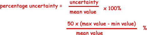
Percentage uncertainty (of a mean value)

When you analyse your results you take a 'mean value' of each set of readings for your chosen independent variable value. To work out the percentage of its uncertainty you need to use the following equation:

Suppose you had calculated three readings for the period of swing:

1.06s 1.07s 1.05s

The percentage uncertainty would be:

50 x (1.07 - 1.05)/1.06 = 0.943%

When two values are multiplied together (or divided) you add the uncertainty percentages for them together,

Suppose the uncertainty of X was 0.2% and the uncertainty of Y was 0,7% - then the uncertainty of XY would be 0.9%

In the write-up of a full practical report calculation of uncertainties can be tedious (MS-Excel can be useful for this!)

In examinations they usually get you to work out the uncertainty of one set of readings - not a whole table. Make sure you do the correct one!

Plotting Graphs

The commonest mistake is in not labelling the axes properly - there should be a physical quantity and its units - remember if you square a physical quantity its unit is squared too... and logs, sines etc have no unit as they are ratios....

Each graph should have a title - even if it is just the question number part..

The graph must fill the graph paper. If the examiner could double the size of any of your axes and still get the readings on the graph paper you lose marks!

Points should be neat crosses.

Lines should be smooth, fine and clearly visible. Straight lines should be made with a long ruler!

Text should be in ink - lines in pencil.

Calculating the gradient

The sides for the triangle to calculate a gradient should be large (for AQA large is bigger than 8 cm!). Label the vertices ABC and spell out what you are doing - don't take short cuts!

The gradient of the graph is y/x